Abstract
The Large Synoptic Survey Telescope (LSST) plans to produce a live stream of its detections of transient astronomical events within 60 seconds of observation at an expected rate of about 10,000 alerts per visit and 10 million per night. According to the VOEvent database archived by 4piSky, existing technology supports a current alert stream rate of ~43,000 per month. Additionally, the LSST alerts are expected to be significantly larger in size than past alerts given the plan to include cutout “postage stamp” images with each alert event packet. In anticipation of supporting an alert stream unprecedented in size and velocity, we are experimenting with streaming technology that is used at large scale outside of astronomy that may be suitable for our use case. Here we benchmark the performance of an alert distribution testbed using this streaming technology.
Introduction
Current performance requirements on the LSST alert system expect to distribute at minimum nAlertVisitAvg = 10,000 alert events every 39 seconds, with a stretch goal of supporting 100,000 per visit.
This minimum averages to ~250 alerts per second, though may be transmitted at a higher, much more bursty rate, compared to the current VOEvent rate of ~1 alert per minute.
The LSST alerts are planned to contain a significant amount of information in each alert event packet,
including individual event measurements made on the difference image, a measure of the “spuriousness” of the event,
a limited history of previous observations of the object associated with the event if known, characteristics of the variability of the object’s lightcurve,
the IDs and distances to nearby known objects, and cutout images of both the difference image and the template that was subtracted.
The experiments here use a template alert event packet as described below with very limited content (e.g. no history) with a size of 136 KB, primarily dominated by the 90 KB size of the two cutout images in FITS format.
A full alert packet with all event measurements and a history of previous observations will be larger.
On the receiving end of the alert distribution system will be community brokers and a limited filtering service mini-broker.
The LSST filtering service is expected to be able to support numBrokerUsers = 100 simultaneous connected users each receiving at most numBrokerAlerts = 20 full alerts per visit.
In order to meet LSST’s alert stream needs, the alert distribution system must be able to scale to support the expected volume of the alert stream, to support the number of connections, and to allow filtering capabilities that can be made user friendly with simple Python or SQL-like language.
Here we test the scalability of a preliminary mock alert distribution system testbed.
Technology Suite
For alert distribution, serialization, and filtering, we are testing primarily three open source technologies supported by the Apache ecosystem: Kafka, Avro, and Spark.
Kafka
For alert distribution, we are testing Apache Kafka. Kafka is a logging system or messaging queue reinvented as a distributed streaming platform. It is highly-scalable and used in production at companies like LinkedIn, Netflix, and Microsoft to process over a trillion messages per day. Originally out of LinkedIn, the development of Kafka is supported by the company Confluent, which also provides an ecosystem of tools around Kafka. The Kafka ecosystem has well-supported clients in a number of languages including C/C++ and Python.
Avro
For alert formatting, we are using Apache Avro.
Avro is a data serialization system similar to Thrift or Protocol Buffers that provides more structure to data than XML or JSON.
Avro uses schemas, similar to a CREATE TABLE SQL database statement, defined with JSON to describe data structures and data types.
Postage stamp cutout files can be included in alert packets as bytes type.
Spark
For alert filtering, we are experimenting with Apache Spark. Spark is a computing platform in the Hadoop ecosystem for big data. The key relevant feature for this work is Spark Streaming, which allows a simple way to write streaming applications in way similar to tradition batch jobs. Spark Streaming allows for alert filters to be written in simple familiar Python and can be natively connected to Kafka. The initial benchmarking results here do not include filtering with Spark, but we mention it here for because of its fit in the choices for the overall ecosystem.
Benchmarking Experiments
To construct a testbed, we built a containerized suite of simple alert “producers” and “consumers” that serializes an example alert event and talks to a Kafka broker.
Tooling
The main testbed of alert consumers and producers to Kafka can be found in the lsst-dm organization’s “alert_stream” GitHub repo. This repo provides instructions for a Docker build and a Dockerized deployment of Kafka and Zookeeper from the Confluent Platform version 3.2.0. The example alert data and schemas for Avro serialization are pulled into the main Docker image and can be found in lsst-dm organization’s “sample-avro-alert” GitHub repo, including postage stamp cutout files in FITS format. Examples of how to use Spark Streaming with Avro and Kafka can be found in the lsst-dm organizations’s “filtering-blueprints” GitHub repo.
For monitoring the ecosystem deployment with Docker Swarm, we used “swarmprom”, a monitoring suite for Docker Swarm that uses Prometheus, Grafana, cAdvisor, Node Exporter and Alert Manager.
Initial Benchmark
As a first benchmark, we deployed one Kafka broker and one Zookeeper listening to a single alert producer serializing and sending 1,000 alerts (~rate expected from the Zwicky Transient Facility) repeatedly every 39 seconds with two alert consumers on the receiving end of the alerts for 1000 visits or 1 million total alerts. This ZTF scale test will be supplemented by larger scale tests to derive scaling curves. Note well that we use the term “broker” here to mean a broker in the sense of Kafka nodes, whereas any references to the LSST mini-broker alert filtering system explicitly use the term “mini-broker.”
The system was run on Amazon’s Web Services (AWS) using the Docker for AWS CloudFormation Template. The Docker Swarm size was set to a cluster of 3 Swarm managers and 5 Swarm worker nodes. All managers and workers were set to r3.xlarge EC2 HVM instance size with 200 GiB standard ephemeral storage. The r3.xlarge flavor is a memory optimized flavor with 4 vCPUs, 2.5 GHz, Intel Xeon E5-2670v2, and 30.5 GiB memory.
Results
For one producer generating 1000 alerts per visit x 1000 visits with two consumers (consumer1 counts all and prints every 100th alert and consumer2 just prints the latest offset from Kafka), no alerts were lost in transit. The average time for 1000 alerts to be generated, sent to Kafka, and received by the consumer was ~4.2 seconds.
Timing Mean +/- Stddev Min-Max Producer serialization and send to Kafka 3.88 +/- 0.25 s 3.37 - 4.32 s Transit time to receipt by consumer 0.30 +/- 0.23 s 0.06 - 1.05 s
The following measurements were derived from observations output every 5 minutes over the ~11 hours of generating 1 million alerts.
CPU (%) Mean +/- Stddev Max Kafka 9.0 +/- 3.8 39.0 Zookeeper < 0.1 +/- 0.1 1.3 Producer 23.9 +/- 6.4 44.8 Consumer1 8.3 +/- 2.4 15.6 Consumer2 0.1 +/- 0.1 0.6
Memory (GiB) Mean +/- Stddev Max Kafka 26.1 +/- 6.6 30.6 Zookeeper 0.08 +/- 0.01 0.08 Producer 0.02 +/- 0.02 0.09 Consumer1 0.009 +/- 0.0004 0.015 Consumer2 0.008 +/- 0.0002 0.009
Network in Mean +/- Stddev Max Kafka 2.08 +/- 0.58 MiBps 3.6 MiBps Zookeeper 81 +/- 97 Bps 1.2 KiBps Producer 11 +/- 3.3 KiBps 24.8 KiBps Consumer1 2.05 +/- 0.59 MiBps 3.5 MiBps Consumer2 2.01 +/- 0.56 MiBps 3.5 MiBps
Network out Mean +/- Stddev Max Kafka 4.03 +/- 1.10 MiBps 7.0 MiBps Zookeeper 49 +/- 79 Bps 966 Bps Producer 1.97 +/- 0.54 MiBps 3.5 MiBps Consumer1 23.7 +/- 6.5 KiBps 43.4 KiBps Consumer2 2.01 +/- 0.56 MiBps 3.5 MiBps
Cluster total IO Mean +/- Stddev Max read 1.25 +/- 4.27 KiB 75.2 KiB written 2.5 +/- 3.4 MiB 61.0 MiB
Cluster total network traffic Mean +/- Stddev Max received 6.4 +/- 1.0 MiBps 6.8 MiB transmitted 6.5 +/- 1.0 MiBps 6.8 MiB
The networking traffic pattern shows some burstiness seen in Figure 1. The bandwidth out is higher than in because this experiment has two consumers reading the full stream.
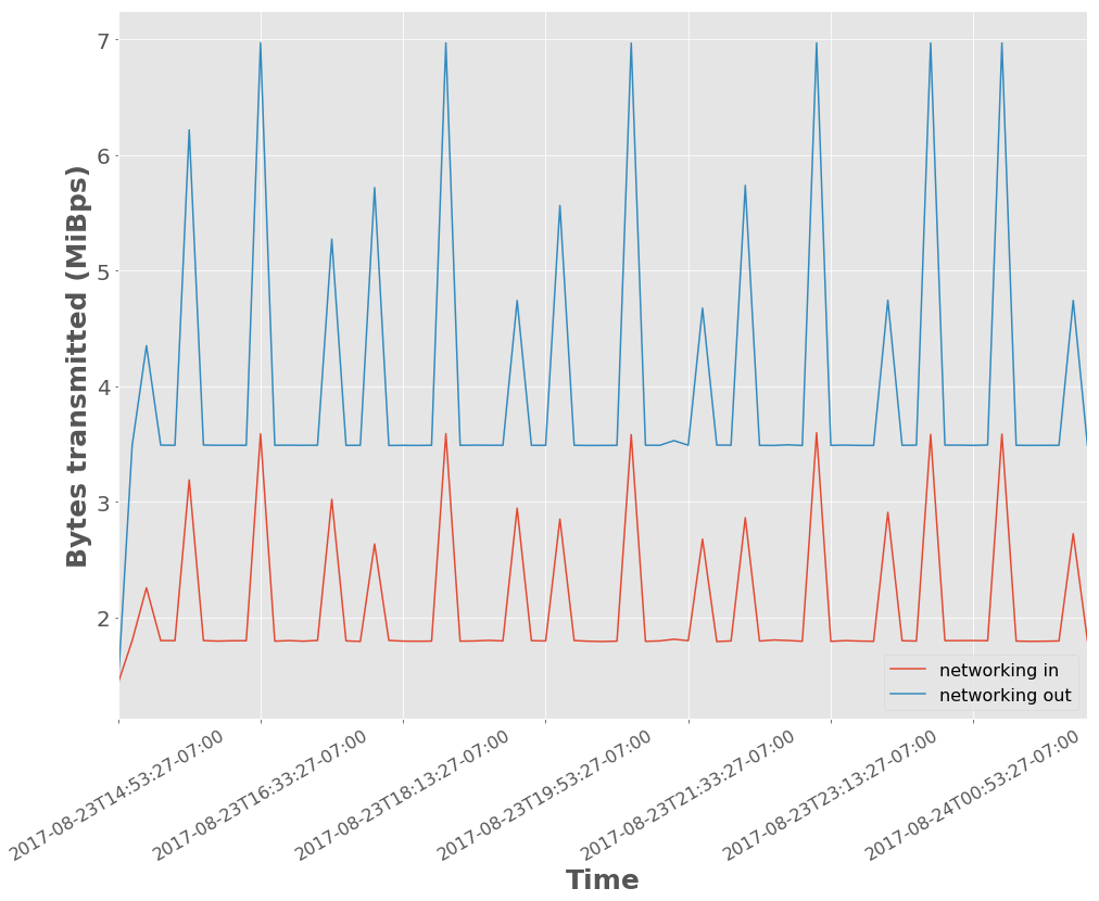
Figure 1 Network traffic in and out of Kafka. The x-axis ticks are demarcated at time intervals of 1 hour and 40 minutes.
Scaling Alert Volume
To complement the initial benchmarking experiment at ZTF scale and derive scaling curves, we ran several similar tests varying the total number of alerts produced per visit. We set the alert producer to serialize and produce 100, 1,000, and 10,000 alerts per visit and also ran each of those tests once including and once without including the postage stamp cutout files in the alert packets to further vary the volume of data sent per visit. The tests use the same testbed setup as the initial benchmark experiment, using Docker for AWS as described above, with again 3 Swarm managers and 5 Swarm worker nodes on r3.xlarge machines. For the larger experiments, we increased the instance ephemeral storage to the maximum of 1 TiB.
Results
Given the results from the initial benchmark, the most interesting metrics or where the Kakfa system uses a significant amount of resources are the timing metrics for serialization and for transportation of alerts, memory usage for Kafka, and network traffic in and out of the Kafka system.
In Figure 2 and Figure 3, we show the mean time it takes to serialize into Avro format and send a batch of alerts to Kafka. 100 alerts takes about 1 second to serialize and send to Kafka, 1,000 alerts takes about 3-4 seconds, and 10,000 alerts takes about 28-33 seconds for a single producer. A single producer then can serialize about 300 alerts into Avro per second.
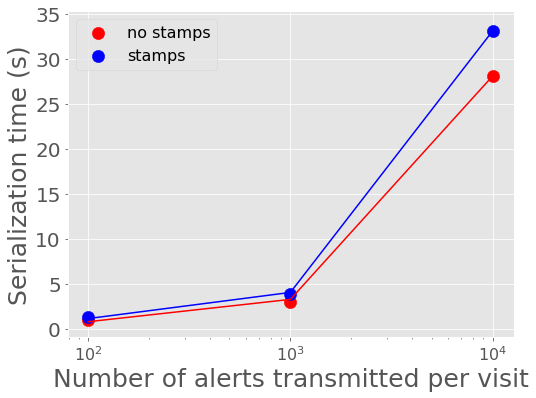
Figure 2 Alert serialization time vs number of alerts in a batch with best fit linear relations overplotted.
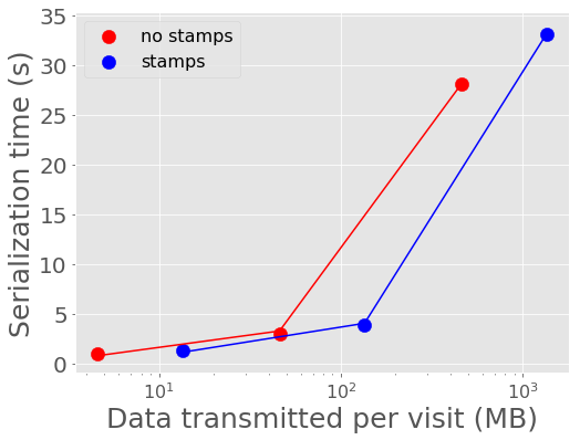
Figure 3 Alert serialization time vs volume of alerts with best fit linear relations overplotted.
Figure 4 and Figure 5 show the mean time it takes for the last alert in a batch produced to be sent through Kafka and received by a consumer. For all experiments, the transport time is low, between 0.10 - 0.30 seconds. The time spent serializing alerts into Avro format on the producer end dominates over the transport time.

Figure 4 Alert transit time vs number of alerts in a batch with best fit linear relations overplotted.
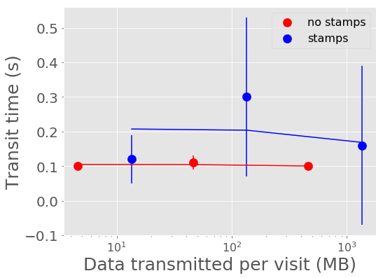
Figure 5 Alert transit time vs volume of alerts with best fit linear relations overplotted.
Figure 6 and Figure 7 show the average memory usage by Kafka over the length of each experiment. A back-of-the-envelope calculation for estimating memory needs says that if you want Kafka to buffer for 30 seconds then the memory need is write_throughput*30. If we say on average the alert throughput is at least 250 alerts/second (but really bursty and likely higher) then the memory estimate is 250 alerts/sec * 135 KB/alert * 30 seconds = 10+ Gigabytes. Memory usage increases more rapidly with data volume for the larger single alert size (including postage stamps), nearing the maximum for the compute instance size for 1,000 and 10,000 alerts per visit with stamps.
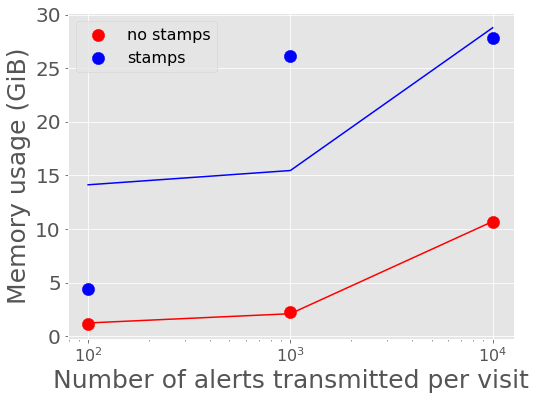
Figure 6 Kafka memory usage vs number of alerts in a batch with best fit linear relations overplotted.
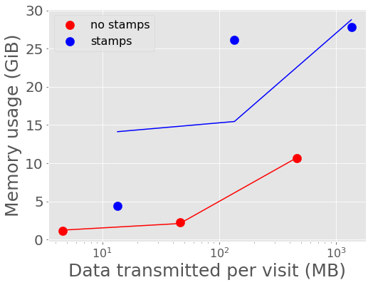
Figure 7 Kafka memory usage vs volume of alerts with best fit linear relations overplotted.
Figure 8 - Figure 11 show the peak network traffic in and out of the Kafka broker. For 10,000 alerts, the alert producer creates a peak of 23 MiBps into Kafka, and the two consumers double the network traffic out at 45 MiBps.
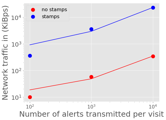
Figure 8 Network traffic into Kafka vs number of alerts in a batch with best fit linear relations overplotted.

Figure 9 Network traffic into Kafka vs volume of data in a batch with best fit linear relations overplotted.
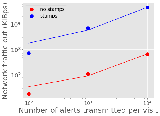
Figure 10 Network traffic out of Kafka vs number of alerts in a batch with best fit linear relations overplotted.
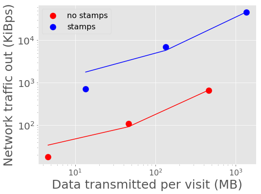
Figure 11 Network traffic out of Kafka vs volume of data in a batch with best fit linear relations overplotted.
Scaling Alert Producers
We ran several simulations increasing the total number of alert producers, holding all else constant, again with two consumers, one consumer counting and printing every 100th alert and one consumer used for the timestamps which prints only the latest offset upon reaching the end of the topic’s partition (i.e., when there are no more alerts to read.) We tested 1, 10, 100, and 200 alert producers serializing and producing in total 10,000 alerts per visit (e.g., 200 alert producers each producing 50 alerts.) Assuming 189 CCDs for LSST and a unit of pipeline compute parallelization per CCD, the experiment with 200 producers each producing 50 alerts is most similar to what we might expect in practice. We also ran each of those tests once including and once without including the postage stamp cutout files in the alert packets. The tests use a similar testbed setup as the initial benchmark experiment, using Docker for AWS as described above, but with 3 Swarm managers and 10 or 15 Swarm worker nodes on r3.xlarge machines to allow for the additional producer containers.
Results
For the performance metrics measured for the Kafka container, particularly memory and network traffic in and out, there is no significant difference between the values for a single alert producer producing 10,000 alerts per visit and an increased number of producers. Increasing the number of producers does make a measurable difference for the time to serialize 10,000 alerts and for end-to-end transport time.
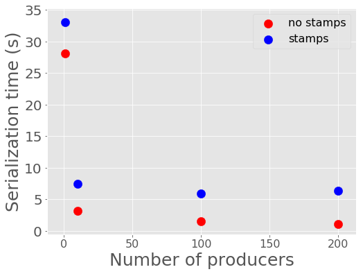
Figure 12 Alert serialization time vs number of producers serializing a total of 10,000 alerts.
The time to serialize and send alerts to Kafka decreases with the number of producers, essentially a reflection of the parallelization of the task with a small additional overhead. One producer serializing 100 alerts takes 1.29 +/- 0.06 seconds, whereas 100 producers serializing and sending 100 alerts each to Kafka takes 5.9 +/- 1.3 seconds.
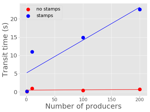
Figure 13 Alert transit time vs number of producers with best fit lines overplotted.
The transit time between when a visit of alerts is finished sending to Kafka and when a consumer has finished reading to the end of the topic’s partition
increases significantly with additional producers for the simulations which include postage stamp cutouts in the alert packets.
For one alert producer with and without stamps and for all simulations without stamps, the transit time is less than 1 second.
For 200 producers with 50 alerts each with stamps, the average transit time for a visit of alerts increases to 22.6 seconds.
Because of the difference between experiments including stamps and excluding stamps, there may be a configuration change necessary
that is related to the average message size.
One potential configuration parameter to experiment with tuning is the producer batch.size, which has a default size of 16384 bytes,
smaller than a single alert message.
Scaling Alert Consumers
In testing an increased numbers of consumers, we encountered issues with the default Kafka settings and a single producer producing 10,000 alerts. The increased of number of consumers slowed the producer’s submission of alerts to the Kafka queue so much as to lag behind the 39 second pause between bursts of alerts from sequential visits. Instead of a single producer, we used 10 producers each producing 1,000 alerts, and we increased the Java heap size of Kafka to 8 GB. We also used a more powerful AWS cluster for our Docker Swarm. We used 3 Swarm managers on m4.16xlarge instances (64 vCPUs, 256 GiB memory, and 10,000 Mbps EBS bandwidth) and 10 worker nodes on m4.4xlarge instances (16 vCPUs, 64 GiB memory, and 2000 Mbps EBS bandwidth) all with 1 TiB of ephemeral storage. When initiating Kafka and the alert stream component containers, we made sure to constrain the Kafka container to its own node and separate the other containers to different nodes so as not to have Kafka competing with other containers for resources. With these settings, the lagged producer problem is resolved. In practice for the expected LSST alert distribution system in production, this will likely not be a problem since there should be one producer per CCD, with the planned compute parallelization of the pipeline.
Results
For scale testing of consumers, we performed four different tests, one with two consumers, one with four, one with six, and one with eleven. In each test, all but used one consumer processes the stream by printing every 100th alert and the remaining consumer reads the stream and just drops the messages. Each of the four tests were run both with postage stamps and without, for a total of eight tests.
Below shows the memory utilization of Kafka with an increased number of consumers and larger allotted instances on AWS.

Figure 14 Kafka container memory utilization against number of consumers.
During testing for the two consumer test, instances were only allotted 32 GiB of memory. While debugging slow performance with multiple consumers, we increased the available memory to 256 GiB and observed that Kafka then utilized more memory. Tests with stamps included in alerts are significantly more memory intensive for Kafka than tests without including postage stamps cutouts.
For these tests there is no difference for the network traffic into Kafka, as we are still sending 10,000 alerts in each visit burst. The network traffic out of Kafka increases linearly with more consumers, as expected, up to 180000 KiBps (180 Mbps) for 10+1 consumers, since each consumer pulls its own stream.

Figure 15 Network traffic out of Kafka against number of consumers.
Below shows the length of time it takes for producers to serialize alerts into Avro and produce to the Kafka broker. In the case of one producer serializing the full alert stream, increasing consumers has a very large effect on the producer speed, lagging the end-to-end process. After increasing to ten producers, as shown, below, having more consumers has a smaller impact on the producer time. The serialization and producing time increases slightly and near linearly to 9 seconds. With more producers producing in parallel (one per CCD), this number would likely be lower.
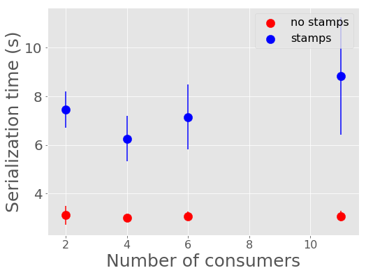
Figure 16 Serialization and Kafka submission time for producers against number of consumers.
The transit time of alerts, the time it takes for alerts to be read by the consumers after they have been submitted into the Kafka queue, increases with number of consumers. Below shows the relationship between the transit time and number of consumers.
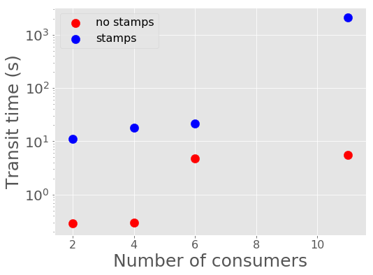
Figure 17 Transit time of alerts to consumers against number of consumers.
For the test with 10+1 consumers including postage stamp cutouts, the average transit time is very large. The consumers are unable to keep up with bursts of alerts every 39 seconds. Below shows the transit time lag increasing for alert bursts for 300 visits.
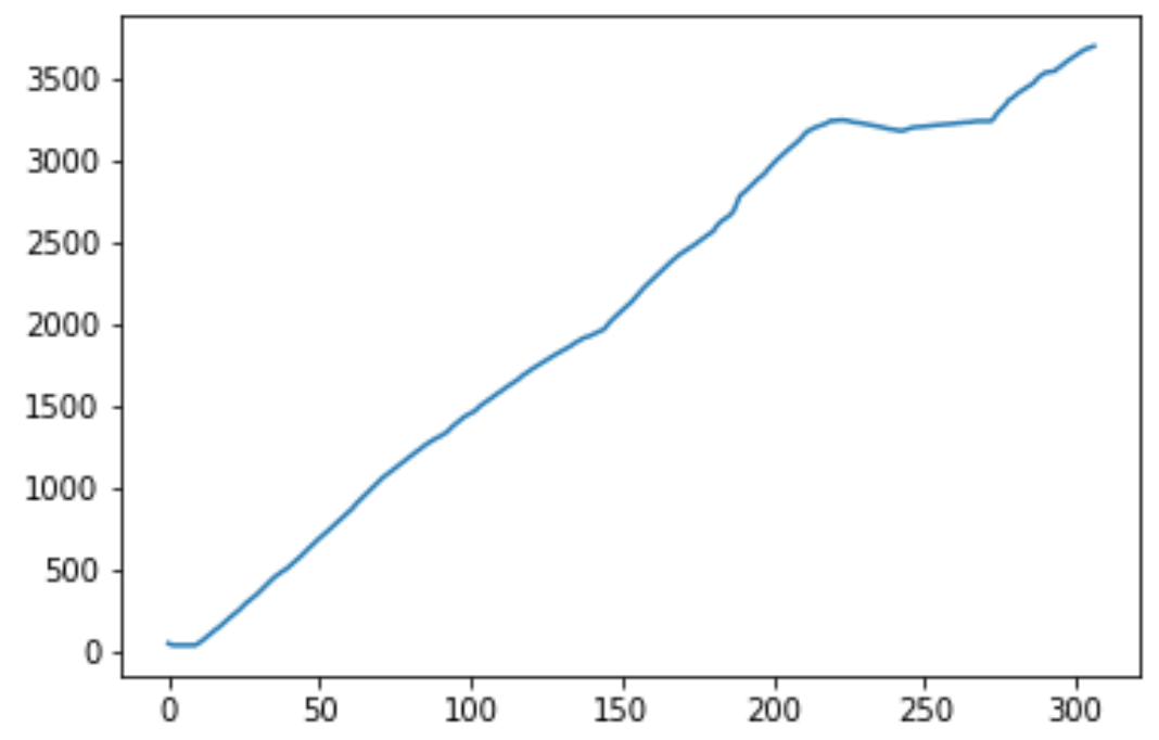
Figure 18 Length of time from Kafka to consumer receipt and processing in seconds (y axis) vs. visit number (x axis).
Fortunately, even with the very slow consumer read time, the producer submission time does not appear to be affected with the number of parallel producers increased to ten.
It is unclear why an increased number of consumers would significantly slow a single producer as to be unable
to keep up with the 39 second separation between bursts. With larger instance sizes, there should be no bottleneck
in reading from disk and no bottleneck in the total network traffic. Though the parallelization of compute per CCD, i.e.,
an increased number of producers in parallel, should eliminate this problem, there is the possibility of
performance improvement if this issue can be addressed. Preliminary testing indicates that adjusting three
parameters, buffer.memory, batch.size, and linger.ms, together may help. Using multiple partitions
may also help. All tests above use a single partition for a single topic.
It is also unclear why the consumers consumption time is slowed for the case of 10+1 consumers reading a stream with stamps. The consumer consumption time is outside the total alert production pipeline time for the alerts to be accessible from Kafka, and a slow consumer can have additional processing while reading the stream that can slow the process, but the transit and consumption time should still be considered. Consumer reading of the stream can easily be parallelized for faster processing. The parallelization is controlled by the number of topic partitions, so increasing the number of partitions can decrease consumer read time such that consumers do not lag behind bursts if the consumers read in consumer groups in parallel, which we explore below. For the critical time from producer serialization into Avro and submission to Kafka, the time it takes for the alert distribution to get alerts into the queue and ready to be read by consumers can be expected to be about 6-9 seconds when stamps are included and 1-3 seconds without stamps.
Parallelization with Multiple Partitions
The alert stream we are using is pushed to a single “topic” within Kafka, into which alert messages are queued. Kafka topics can then be divided into a number of “partitions,” each of which can be placed on separate machines to allow for multiple consumers to read from a topic in parallel. We constructed a testbed for multiple partitions using an AWS Docker Swarm cloud of 3 Swarm managers on m4.16xlarge instances (64 vCPUs, 256 GiB memory, and 10,000 Mbps EBS bandwidth) and 10 worker nodes on m4.4xlarge instances (16 vCPUs, 64 GiB memory, and 2000 Mbps EBS bandwidth) all with 1 TiB of ephemeral storage, as before. This simulation used a Kafka cluster of 3 brokers configured to have an alert stream topic with 10 partitions, allowing consumers to parallelize into 10 consumer feeds. The Kafka containers were constrained to manager nodes and separated from the other alert stream producing and consuming containers. We used 100 containers for producers, each producing 100 alerts in bursts every 39 seconds. On the consumer side, we used 10 consumer groups each printing every 100th alert and 1 consumer group dropping alerts and printing only end of partition notices (i.e., a message that there are no more alerts to read) for monitoring. Each consumer group consisted of 10 individual consumers acting in parallel to consume the full stream.
Results
Using a 3-broker Kafka cluster, multiple partitions, and consumer groups decreases the total time to distribute alerts, from initial Avro serialization of alerts to consumer receipt. No significant difference from previous experiments of the compute resource utilization is observed. The impact observed in previous simulations of an increased number of consumers slowing the time to produce alerts is lessened. In this case, with 11 consumer groups reading a full stream each, the time to serialize one visit of alerts and send the batch to Kafka is less than the experiment with only two consumers and a single partition. In the previous experiment with 11 consumers and one partition, the consumers were unable to keep up with the alert stream visits and fell increasingly behind. With 10 partitions and the same number of consumer groups, the transit time of the consumer reading alerts from the Kafka queue is ~11 seconds.
Below is a table of simulations ordered from the smallest total alert distribution duration to largest. Generally, having more consumers (with only a single partition) increases the total distribution time, primarily affecting the consuming time, and parallelizing into multiple producers decreases the serialization and producing time. Multiple partitions decreases both time on the consumer end and on the producer end.
| Experiment | Producing Time (s) | Consuming Time (s) | Total |
|---|---|---|---|
| 100 producers, 11 consumers, 10 partitions | 3.75 +/- 1.30 | 10.8 +/- 3.52 | 14.55 |
| 10 producers, 2 consumers, 1 partition | 7.46 +/- 0.23 | 11.0 +/- 2.0 | 18.46 |
| 100 producers, 2 consumers, 1 partition | 5.9 +/- 1.3 | 14.9 +/- 1.3 | 20.8 |
| 10 producers, 4 consumers, 1 partition | 6.26 +/- 0.93 | 17.91 +/- 3.33 | 24.17 |
| 10 producers, 6 consumers, 1 partition | 7.15 +/- 1.34 | 21.14 +/- 2.17 | 28.29 |
| 1 producer, 2 consumers, 1 partition | 33.1 +/- 2.02 | 0.16 +/- 0.23 | 33.26 |
| 10 producers, 11 consumers, 1 partition | 8.82 +/- 2.41 | 2068 +/- 1131 | 2077 |
Conclusions
Compute Resources and Settings Recommendations
For a robust alert distribution service, a cluster of at least three Kafka brokers and a replication factor of two is recommended. However, we did not test here the performance effects of a replication factor greater than one.
Kafka is a memory intensive application. In the experiments here, each Kafka broker tends to utilize all
available memory, which it needs to buffer events from active producers.
In terms of hardware recommendations, Confluent, the main contributor to Kafka, recommends a machine with
64 GB of RAM or an AWS instances with 32 GB. An appropriate back of the envelope calculation to determine
hardware needs is write_throughput *30 if you want a 30 second buffer. If we assume one alert is ~135 KB
and possible bursts of up to 10,000 alerts/second, that is equivalent to 1.35 GB/second. If we want to buffer
for between 30-60 seconds, given the time between visits, an appropriate memory range is then between ~40-80 GB.
In all experiments above, Kafka tends to be low on CPU requirements. It is noted by Confluent that enabling SSL can significantly increase the CPU requirements. A reasonable recommendation is for 24 core machines.
The requirements for storage disk sizes depend on the amount of time we will cache / allow “rewindable” access to the alert stream and the number of partitions configured for each topic. If all alerts are streamed out in a single topic and the alert sizing assumptions here are correct, one night of minimal alerts is about ~1.5 TB. Each partition of a topic must fit on its own disk, and it is recommended that these disks are dedicated to the Kafka service. The number of partitions sets the maximum number of readers that can be parallelized in a single consumer group. A reasonable choice would be to start a new “topic” each day, which would allow rewinding to the beginning of the night. Below shows the minimum disk size and the total number of those disks needed for different numbers of partitions and cache length assumptions for a replication factor of one. Fewer disks of larger size are also fine as long as no partition is forced to be split over multiple disks. The file system used should be POSIX compliant.
| Cache/Rewind time allowance | Partitions/Parallel consumers | Disk space (num disks x size) |
|---|---|---|
| 1 day | 1 | 1 x 1.5 TB |
| 1 day | 16 | 16 x 94 GB |
| 1 day | 32 | 32 x 47 GB |
| 1 day | 64 | 64 x 24 GB |
| 1 day | 128 | 128 x 12 GB |
| 7 days | 1 | 1 x 10.5 TB |
| 7 days | 16 | 16 x 656 GB |
| 7 days | 32 | 32 x 328 GB |
| 7 days | 64 | 64 x 164 GB |
| 7 days | 128 | 128 x 82 GB |
| 14 days | 1 | 1 x 21 TB |
| 14 days | 16 | 16 x 1.3 TB |
| 14 days | 32 | 32 x 656 GB |
| 14 days | 64 | 64 x 328 GB |
| 14 days | 128 | 128 x 164 GB |
| 30 days | 1 | 1 x 45 TB |
| 30 days | 16 | 16 x 2.8 TB |
| 30 days | 32 | 32 x 1.4 TB |
| 30 days | 64 | 64 x 703 GB |
| 30 days | 128 | 128 x 352 GB |
In the experiments here, an increased number of partitions decreases the total time to distribute alerts on both the producer and consumer side and allows consumers to use parallel readers. A number of partitions greater than one is recommended, and if the compute pipeline is parallelized by CCD, one partition per CCD, would be a reasonable choice. More partitions can lead to higher throughput but requires increased memory. As a rule of thumb, Confluent recommends no more than 100 * b * r partitions per broker, where b is the number of brokers and r is the number of replications. For a three-broker cluster and a replication of a two, the limit is then 600 partitions.
General Suitability
Kafka provides a number of advantages for use as an alert data distribution system. Data can be easily replicated, and the system can be easily scaled to handle a higher load by adding additional brokers. The experiments here utilize Docker containers for deploying Kafka, and scaling the number of brokers in the system involved simply 1) deploying each broker as a separate container, 2) configuring each broker to connect to the instance of Zookeeper, and 3) ensuring that each broker was given a separate ID.
The Kafka system is able to handle a data volume and throughput similar to what is expected for the LSST pipeline. We have used here Avro alerts of comparable size to an LSST alert with one detection and including postage stamp cutouts with bursts of 10,000 alerts every 39 seconds in experiments running up to 11 hours and encountered no data loss. On the producer side, we were able to parallelize the alert serializers producing to Kafka, and the increased connections did not have a noticeable detrimental effect on the system. On the consumer side, we were also able to successfully parallelize the consumers into 10 groups of 10 (100 total stream readers), each group pulling the equivalent of 10 streams of data. With our largest experiment with a configuration closest to the stress of the actual expected LSST pipeline (100 producers, 10*10 consumers, 10 partitions), we were able to serialize and submit batches of 10,000 alerts to the alert distribution queue in 3.75 +/- 1.30 seconds, 6.25% of the total 60 second end-to-end pipeline constraint. Additional producers (one per CCD) may decrease the total time further. Consumer groups acting in parallel were then able to pull and process (apply a very simple filter) to the alerts in an additional 10.8 +/- 3.52 seconds.
The most significant issue thus far is that the volume of data will quickly saturate the available network bandwidth as the number of consumers (and e.g., filter processes) increases, if parallelization of consumers can not be achieved. Parallelizing alert filter consumers in the mini-broker is yet to be explored. Assuming that the size of alerts has been estimated accurately, an Avro serialized alert for a source with a single detection and no history is about 140 KB. Approximately 2/3 of the size of an alert with no history is due to the postage stamps for the template and difference image, assuming FITS files with 30 x 30 pixels. For most experiments and metrics measured, there is a noticeable impact on Kafka compute utilization, end-to-end timing, and, particularly, utilized bandwidth when postage stamp cutouts are included in the alert packets due to the large size. The inclusion of postage stamp cutouts is currently a science requirement. However, results here suggest that additional consideration be given to alternatives for the distribution of stamps, if it is possible that the current requirements may be adjusted. One alternative to including postage stamps in the stream, recommended by other users of Kafka for large messages, is to forego including the stamps in the stream and instead include a url to the location of the stamps from which the stamp can be accessed separately. This would particularly alleviate the increased network traffic for each additional consumer reading a stream. Another potentially possible alternative could be to separate the postage stamps into their own Kafka topic. If not all primary consumers are required or expected to read postage stamp cutouts and pass them to downstream users, this could decrease the total network traffic. Not all consumers would need to pull from the larger stream of stamps. A downstream filter could then unite alerts of interest with corresponding stamps. The feasibility of this option for combining streams still needs to be further investigated.